
As a model of line spread of slanted edge consider the function
where 

Fig 1a
 |
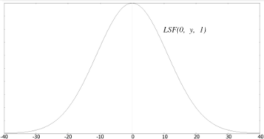 |
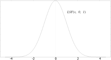
| Fig 1b | Fig 1c |
Fig 1a - LSF with sigma = 1 and k = 0.09; Fig 1b - xz section at y = 0; Fig 1c - yz section at x = 0;
Consider applying 2d Gaussian blur with sigma = to
to
 . Regarding
the Gaussian blur's separability we can represent it as two sequenced
convolutions in x and y directions:
. Regarding
the Gaussian blur's separability we can represent it as two sequenced
convolutions in x and y directions:

Eq. 1
Gaussian blur has two more properties:

and
Tilde means equality up to an intensity scaling constant. The constant doesn't matter in our case because we always scale the LSF to fit in range [0..1].
Using the mentioned properties we can rewrite Eq. 1:

Thus, applying 2d Gaussian blur with sigma =
to 'ideal' slanted edge
is similar to applying 1d Gaussian blur with sigma =
 to every scan
line, where k is the edge slope.
to every scan
line, where k is the edge slope.
Oleg Kurtsev (okurtsev@quickmtf.com)